For our two-class ( DNA -binding and non-binding residues) classification problem, we applied three machine learning algorithms: support vector machine ( SVM ) (Vapnik, 1998), kernel logistic regression (KLR) (Zhu and Hastie, 2005), and penalized logistic regression ( PLR ) (le Cessie and van Houwelingen, 1992). SVM is a margin maximizing classifier that does a linear classification in the feature space, which corresponds to a non-linear classification in the original data space. The feature space is obtained by transforming data from the original data space with a kernel function. Similarly, KLR and PLR are also margin maximizing classifiers. Optimization problem of KLR and PLR is also similar to that of SVM , except that they use exponential loss function instead of L1 loss function of SVM . Both KLR and PLR provide classification results based on conditional class probability. The difference is that PLR does the classification in the original data space, whereas KLR does the classification in the feature space by using a kernel function. In other words, KLR is a non-linear version of PLR . For both SVM and KLR we used the radial basis function kernel, which showed the best performance on our dataset.
We used leave-one-protein-out cross-validation to train and test each classifier. In this procedure, 61 protein complexes are used for training and the remaining one complex is used for testing. This process is repeated 62 times so that each protein complex can be tested. Optimal parameters in a classifier were determined to be those which achieved the best average accuracy across the 62 cross-validation experiments. To assess the given classifier's performance, we computed mean and standard deviation of the following performance measures across the 62 cross-validation experiments:
(i) accuracy: ACC=(TP+TN)/(TP+FP+TN+FN)
(ii) sensitivity: SN=TP/(TP+FN)
(iii) specificity: SP=TN/(FP+TN)
Where TP is the number of true positives (correctly predicted DNA -binding residues), FN is the number of false negatives ( DNA -binding residue predicted as being non-binding), TN is the number of true negatives (correctly predicted non-binding residues), FP is the number of false positives (non-binding residues predicted as being DNA -binding).
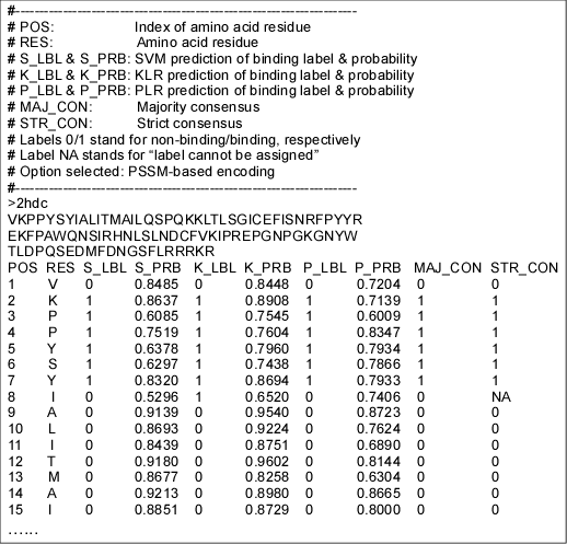
Figure 1. A sample prediction result, consisting of three parts: a header describing its format, inputted FASTA sequence, and a prediction result in a columnar format. The result was truncated to fit the page. Refer to help for details.
Table 1. Performance measures from previous studies. For DBS- PRED , results from SeqPredNet are shown since this version is implemented as the web server. Similarly, results from PDNA- RDN are shown for DBS-PSSM. In three studies (DBS-PRED, DBS-PSSM, and BindN) as well as our current study, specificity is calculated as TN/(FP+TN), whereas it is calculated as TP/(FP+TP) in Yan et al . (2006).
|
Accuracy |
Sensitivity |
Specificity |
DBS-PRED (Ahmad et al., 2004) |
64.5 |
68.6 |
63.4 |
DBS-PSSM (Ahmad and Sarai, 2005) |
64.0 |
67.1 |
63.3 |
BindN (Wang and Brown, 2006) |
70.31 |
69.40 |
70.47 |
Yan et al. (2006) |
78 |
44 |
41 |
Table 2. The average accuracy of SVM classifiers tested on the four major structural classes of proteins (the balanced training/test set, for details see Kuznetsov et al, 2006, Proteins). In each cell the fraction of residues predicted correctly is shown.
|
|||||||||||||||||||||||||||||||||||||||||||||||||||||||||||||||||||||||||||||||||||||||||||||||||||||||||||||||||||||||||||||||||||||||||||||||||||||||||||||||||||||||||||||||||||||||||||||||||||||||||
|
|||||||||||||||||||||||||||||||||||||||||||||||||||||||||||||||||||||||||||||||||||||||||||||||||||||||||||||||||||||||||||||||||||||||||||||||||||||||||||||||||||||||||||||||||||||||||||||||||||||||||
|
|||||||||||||||||||||||||||||||||||||||||||||||||||||||||||||||||||||||||||||||||||||||||||||||||||||||||||||||||||||||||||||||||||||||||||||||||||||||||||||||||||||||||||||||||||||||||||||||||||||||||
Figure 2. |
|||||||||||||||||||||||||||||||||||||||||||||||||||||||||||||||||||||||||||||||||||||||||||||||||||||||||||||||||||||||||||||||||||||||||||||||||||||||||||||||||||||||||||||||||||||||||||||||||||||||||
Figure 3. |
Ahmad,S., Gromiha,M.M. and Sarai,A. (2004) Analysis and prediction of DNA-binding proteins and their binding residues based on composition, sequence and structural information. Bioinformatics , 20, 477-486.
Ahmad,S. and Sarai,A. (2005) PSSM-based prediction of DNA binding sites in proteins. BMC Bioinformatics , 6, 33-38.
Kuznetsov,I.B., Gou,Z., Li,R. and Hwang,S. (2006) Using evolutionary and structural information to predict DNA-binding sites on DNA-binding proteins. Proteins , 64, 19-27.
le Cessie,S. and van Houwelingen,J.C. (1992) Ridge estimators in logistic regression. Appl. Statist. , 41, 191-201. [Link]
Vapnik,V.N. (1998) Statistical Learning Theory . John Wiley and Sons, New York .
Wang,L. and Brown,S.J. (2006) BindN: a web-based tool for efficient prediction of DNA and RNA binding sites in amino acid sequences. Nucleic Acids Res. , 34, W243-248.
Yan,C., Terribilini,M., Wu,F., Jernigan,R.L., Dobbs,D. and Honavar,V. (2006) Predicting DNA-binding sites of proteins from amino acid sequence. BMC Bioinformatics , 7, 262
Zhu,J. and Hastie,T. (2005) Kernel logistic regression and the import vector machine. J. Comp. Graph. Stat. , 14, 185-205. [Postscript]